Equations for the free surface

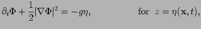
Let us consider motion of a water volume of infinite depth embedded in gravity and bounded by a surface separating it from air at height $z = \eta({\bf x}, t)$ where ${\bf x} = (x,y)$ is the horizontal coordinate. Let the velocity field be irrotational, ${\bf u} = \nabla \Phi$, so that the incompressibility condition becomes

$$\Delta \Phi = 0, \hspace{1cm} \hbox{for\;\;} z < \eta({\bf x}, t).$$ (1)

Rate of change of the surface elevation must be equal to the vertical velocity of the fluid particle on this surface, which gives

$$D_t \eta = \partial_z \Phi, \hspace{1cm} \hspace{1cm} \hbox{for\;\;} z = \eta({\bf x}, t),$$ (2)

where $D_t = \partial_t + {\bf u} \cdot \nabla_\perp$ is the material time derivative. The second condition at the surface arises from the Bernoulli equation in which pressure is taken equal to its atmospheric value. This condition gives

$$\partial_t \Phi + {1 \over 2} \vert \nabla \Phi\vert^2 = - g \eta, \hspace{1cm} \hspace{1cm} \hbox{for\;\;} z = \eta({\bf x}, t),$$ (3)

where $g$ is the free-fall acceleration.

Although equations (2) and (3) involve only two-dimensional coordinate ${\bf x}$, the system remains three-dimensional due to the 3D equation (1). One can transform these equations to a truly 2D form by assuming that the surface deviates from its rest plane only by small angles and by truncating the nonlinearity at the cubic order with respect to the small deviations. This procedure yields the following dynamical equations (see e.g. [17,15]):

$$\eta _{t} = \mathbf{\Gamma }\left[ \Psi \right] \notag$$ (4)

$$-\varepsilon \left( \mathbf{\Gamma }\left[ \mathbf{\Gamma }\left[... ...la _{\bot }\cdot \left[ \left( \nabla _{\bot }\Psi \right) \eta \right] \right)$$ (5)

$$+\varepsilon ^{2}\left( \Gamma \left[ \mathbf{\Gamma }\left[ \mat... ...ot }\left( \mathbf{\Gamma }\left[ \Psi \right] \eta ^{2}\right) \right), \notag$$ (6)

$$\Psi _{t} = -g\eta \notag$$ (7)

$$-\varepsilon \frac{1}{2}\left( \left\vert \nabla _{\bot }\Psi \right\vert ^{2}-\left( \Gamma \lbrack \Psi ]\right) ^{2}\right)$$ (8)

$$-\varepsilon ^{2}\Gamma \lbrack \Psi ]\left( \mathbf{\Gamma }\lef... ...i \right] \eta \right] +\left( \Delta _{\bot }\Psi \right) \eta \right), \notag$$ (9)

where

$$\Psi = \Phi \vert _{z = \eta({\bf x}, t)},$$ (10)

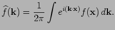
and $\Gamma$ is the Gilbert transform which in the Fourier space corresponds to multiplication by $k = \vert{\bf k}\vert$, i.e.

$$\Gamma \left[ f\right] (\mathbf{x},t)=\frac{1}{2\pi }\int k \wide... ...thbf{k}<tex2html_comment_mark>28 ,t)e^{i\mathbf{k}\cdot \mathbf{x}}d\mathbf{k}.$$

Here, we have the following convention for defining the Fourier transform

$$\widehat{f}(\mathbf{k}) = {1 \over 2 \pi} \int e^{i (\mathbf{k} \cdot \mathbf{x})} f(\mathbf{x}) \, d \mathbf{k}.$$ (11)

In equations (4) and (5), we rescaled variables $\eta$ and $\Psi$ to make them order one, so that the nonlinearity smallness is now in a formal parameter $\epsilon \ll 1$.

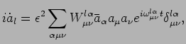
Truncated equations (4) and (5) will be used for our numerical simulations. They have a convenient form for the pseudo-spectral method which computes evolution of the Fourier modes but switches back to the coordinate space for computing the nonlinear terms. However, for theoretical analysis these equations have to be diagonalised in the $k$-space and a near-identity canonical transformation must be applied to remove the nonlinear terms of order $\epsilon$ since the gravity wave dispersion $\omega = \sqrt{gk}$ does not allow three-wave resonances. The resulting equation is also truncated at $\epsilon^2$ order and it is called the Zakharov equation [17,18,19,16],

$$i \dot a_l = \epsilon^2 \sum_{\alpha\mu\nu} { W^{l\alpha}_{\mu\nu... ...a_\alpha a_\mu a_\nu e^{i\omega^{l\alpha}_{\mu\nu}t} \delta^{l\alpha}_{\mu\nu},$$ (12)

where $\omega^{l\alpha}_{\mu\nu} = \omega_l+\omega_{\alpha}-\omega_{\mu}-\omega_{\nu}$, $\omega_l = \sqrt{g k_l}$ is the frequency of mode ${\bf l}$ ( $\; {\bf l} \in {\cal Z}^2$), ${\bf k}_l = 2\pi {\bf l} /L$ is the wavenumber, $L$ is the box size and $k_l = \vert{\bf k}_l\vert$. Here, $a_l$ is the wave action variable in the interaction representation, $a_l = e^{i \omega_l t} b_l$ where $b_l$ is a normal variable,

$$b_l = \sqrt{\omega_l \over 2 k_l} \eta_l + i \sqrt{k_l \over 2 \omega_l} \Psi_l +0(\epsilon).$$ (13)

Here, $0(\epsilon)$ terms appear because of the near-identity canonical transformation needed to remove the quadratic terms from the evolution equations [17,21,16,20,18,19]. Expression for the interaction coefficient $W^{l \alpha} _{\mu \nu}$ is lengthy and can be found in [21].

Zakharov equation is of fundamental importance for theory and it is also sometimes used for numerics. However, in our work we choose to compute equations (4) and (5) because this allows us to use the standard trick of pseudo-spectral methods via computing the nonlinear term in the real thereby accelerating the code.