Next: In what sense are
Up: Probability densities and preservation
Previous: Weak-nonlinearity expansion.
Let us first derive an evolution equation for the generating
functional
 exploiting the separation of the linear
and nonlinear time scales. 3 To do this, we have to calculate
exploiting the separation of the linear
and nonlinear time scales. 3 To do this, we have to calculate  at the intermediate
time
at the intermediate
time  based on its value at
  . The derivation, although
standard for WT, is quite lengthy and will have to be published in a
longer paper. Here, we will only outline the main steps and give the
result. First, we need to substitute the
. The derivation, although
standard for WT, is quite lengthy and will have to be published in a
longer paper. Here, we will only outline the main steps and give the
result. First, we need to substitute the  -expansion of
  from (12) into the expressions
 and
and
 . Second, the phase averaging should be done. Note that, because, we
assume that initial phase factors are independent at with
required accuracy, we can do such phase averaging independently of the
amplitude averaging (which we do not do yet). Thirdly, we take
. Second, the phase averaging should be done. Note that, because, we
assume that initial phase factors are independent at with
required accuracy, we can do such phase averaging independently of the
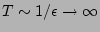
amplitude averaging (which we do not do yet). Thirdly, we take  limit followed by
 (this order
of the limits is essential!). Taking into account that
(this order
of the limits is essential!). Taking into account that
 ,
and
,
and
 and,
replacing
and,
replacing
 by
by  (because the nonlinear time
 we have
Here variational derivatives appeared instead of partial derivatives
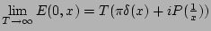
because of the limit. This expression is valid up to the
![$[1+O({\epsilon}^2)]$](img106.png) factor. Equation (15) does not contain
factor. Equation (15) does not contain  dependence which means that that these variables separate from
 's and the solution is a purely-amplitude times an
arbitrary function of 's which is going to be stationary in time.
The latter corresponds to preservation of the initial
's and the solution is a purely-amplitude times an
arbitrary function of 's which is going to be stationary in time.
The latter corresponds to preservation of the initial
 dependence by equation (15) which means that
no angular harmonics of the PDF higher than zeroth will be excited. In
the other words, all the phases will remain statistically independent
and uniformly distributed on
dependence by equation (15) which means that
no angular harmonics of the PDF higher than zeroth will be excited. In
the other words, all the phases will remain statistically independent
and uniformly distributed on  with the accuracy of the equation
(15) integrated over the nonlinear time
with the accuracy of the equation
(15) integrated over the nonlinear time
 , i.e. with
the
, i.e. with
the
 accuracy. This proves the first of the ``essential RPA''
properties. In fact, this result was already obtained before in
[15] for a narrower class of 3-wave systems (see footnote 2).
Note that we still have not used any assumption about the statistics
of
accuracy. This proves the first of the ``essential RPA''
properties. In fact, this result was already obtained before in
[15] for a narrower class of 3-wave systems (see footnote 2).
Note that we still have not used any assumption about the statistics
of 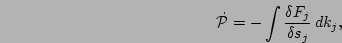 's and, therefore, (15) could be used in future for
studying systems with random phases but correlated amplitudes.
's and, therefore, (15) could be used in future for
studying systems with random phases but correlated amplitudes.
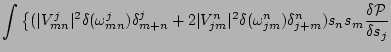
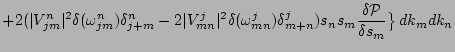
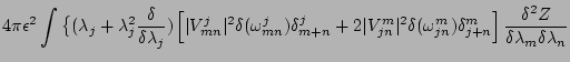
Taking the inverse Laplace transform of (15) we have the
following equation for the PDF,
 |
(15) |
where  is a flux of probability in the space of the amplitude
  ,
,
This equation is identical to the Zaslavski-Sagdeev (ZS) [13]
equation (Brout-Prigogine in the physics of crystals context
[15,16]). Note that ZS equation was originally derived in
[13] for a much narrower class of systems, see footnote 2,
whereas the result above indicates that it is also valid in the most
general case of 3-wave systems. Here we should again emphasize the
importance of the order of limits, first and
 second. Physically this means that the frequency resonance is
broad enough to cover a great many modes. Some authors, e.g. ZS and BP
leave the sum notation in the PDF equation even after the
limit taken giving
second. Physically this means that the frequency resonance is
broad enough to cover a great many modes. Some authors, e.g. ZS and BP
leave the sum notation in the PDF equation even after the
limit taken giving
 . One has to be careful
interpreting such a formula because formally the RHS is null in most of
the cases because there may be no exact resonances between the
discrete
. One has to be careful
interpreting such a formula because formally the RHS is null in most of
the cases because there may be no exact resonances between the
discrete  modes (as it is the case, e.g. for the capillary
waves). Thus, our functional integral notation is a more accurate way
to write the result.
modes (as it is the case, e.g. for the capillary
waves). Thus, our functional integral notation is a more accurate way
to write the result.
Next: In what sense are
Up: Probability densities and preservation
Previous: Weak-nonlinearity expansion.
Dr Yuri V Lvov
2007-01-17
![$\displaystyle 4 \pi {\epsilon}^2
\int \big\{ (\lambda_{j}+\lambda_{j}^2 {\delta...
...delta_{j+n}^{m}
\right]
{\delta^2 Z\over \delta \lambda_{m} \delta \lambda_{n}}$](img103.png)
![$\displaystyle + 2
\lambda_j
\left[ - \vert V_{mn}^j\vert^2 \delta(\omega_{mn}^j...
...a \over \delta \lambda_{n}} \right)
\right]
{\delta Z \over \delta \lambda_{j}}$](img104.png)