


Next: Nonlinear, Non-Rotating Shallow Waters
Up: Hamiltonian formalism for long
Previous: Hamiltonian formalism for long
In non-dimensional form, the shallow-water equations take the form
Here  represents the height of the free-surface, and
  the
horizontal velocity field. The height has been normalized by its
mean value
the
horizontal velocity field. The height has been normalized by its
mean value  , the velocity field
  by the characteristic speed
 (here
(here  is the gravity constant), the horizontal
coordinates by a typical wavelength
is the gravity constant), the horizontal
coordinates by a typical wavelength  , and time by
  . Writing
and assuming that  and
and  are much smaller than one, one
obtains to leading order the linearized equations
are much smaller than one, one
obtains to leading order the linearized equations
At this linear level, the dynamics of waves and vorticity decouple,
with the former satisfying the wave equation, and the latter remaining
constant in time. In particular, if the flow is initially irrotational
(i.e.,
 ), it will remain so forever. Hence
we may restrict our attention here to irrotational flows. These may
be described by a scalar potential
), it will remain so forever. Hence
we may restrict our attention here to irrotational flows. These may
be described by a scalar potential  , such that
For such flows, the system in (![[*]](file:/usr/share/latex2html/icons/crossref.png) , )
reduces to
, )
reduces to
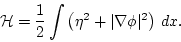
This system is Hamiltonian, with
 |
(5) |
The Hamiltonian form of the equations is
Notice that the Hamiltonian in () is the sum of the
potential and kinetic energy of the system. The former is actually
given by
 , but the difference can be absorbed
by a gauge transformation of the potential . Our goal is to
preserve the essential simplicity of this formulation when we add
nonlinearity, ambient rotation, stratification and vertical shear.
, but the difference can be absorbed
by a gauge transformation of the potential . Our goal is to
preserve the essential simplicity of this formulation when we add
nonlinearity, ambient rotation, stratification and vertical shear.
Next: Nonlinear, Non-Rotating Shallow Waters
Up: Hamiltonian formalism for long
Previous: Hamiltonian formalism for long
Dr Yuri V Lvov
2007-01-17