Testimonials of preveous students

For the summer I was involved in a research project involving the study of Fermi-Pasta-Ulam (FPU) beta-chains. During my time studying under the supervision of Dr. Lvov, I brushed up on classical Lagrangian and Hamiltonian mechanics, studied the numerical solutions of non-linear coupled differential equations, and derived the four-wave kinetic equation amongst other things.

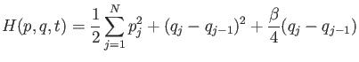
I began my studies by reading a Doctoral Thesis written by Boris Gershgorin. Before this summer, I had not sat down to read a dissertation and was very intimidated by the length and thoroughness of the paper. I was asked to derive the equations of motion from the Hamiltonian, which were in the form of first order differential equations involving p’s and q’s as the dymanical variables. I then expressed the Hamiltonian,

$$H(p,q,t)= \frac{1}{2} \sum _{j=1}^N{} p_j^2 + (q_j - q_{j-1})^2 + \frac{\beta}{4} (q_j - q_{j-1})$$ (1)

in terms of the Fourier conjugates of p and q, such that

$$H(P,Q,t)=\frac{1}{2} \sum _{k=1}^{N-1} \mid P_k \mid ^2 + \omega _k ^2 \mid Q_k \mid ^2$$ (2)

$$+\frac{\beta}{4N} \sum _{k,l,m,s=1} ^{N-1} \omega _k \omega _l \o... ...k Q_l Q_m Q_s^* \delta _s^{klm} +c.c.) + Q_k Q_l Q_m^* Q_s^* \delta _{ms}^{kl}]$$ (3)

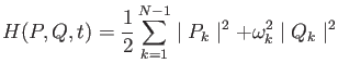
where P and Q are the Fourier conjugates of p and q respectively. Finally, I was told to express the Hamiltonian in terms of variables which were still canonical and analogous to the raising and lowering operators used in quantum mechanics, namely a and a*. So far, I was only required to confirm the conclusions that Boris Gershgorin came to in his thesis, and ensure that I understood that math and concepts.

After doing the derivations, which took about ten pages, I began to have a lot of respect for the amount of time that was put into the dissertation. It wasn’t until doing those ten pages of derivations that I began to understand two or three lines in the thesis. The derivation of those equations was useful because they helped me to review basic Hamiltonian principles, Fourier Transforms, delta functions, and algebraic concepts such the product of multiple sums. Important values which were used in the computations were:

$$\beta = 0.01$$ (4)

$$mass = 1$$ (5)

$$total time \approx 100000$$ (6)

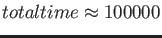
It is important to note that the inital conditions of all the momenta and positions were randomly generated such that the average momentum of all the particles was zero and that the average position was also zero. Additionally, the initial conditions were set so that the initial energy was 50. The accuracy of the energy conservation was not the best. While the initial energy was 50, the ending value of energy was 46.0871. Because of the untilization of the Runge-Kutta integration method, conservation of Energy was not perfect. Yoshida method would have worked more nicely.

I also developed a more intuitive understanding of how creation and annihilation operators corresponded to the creation and annihilation of waves in Fourier space.

Next, I was asked to solve for the equations of motion of a system of

$$N=128$$ (7)

particles. I very much appreciated this part of the research project. The study of non linear FPU chains was most stimulating because, unlike the typical sets of problems that are introduced in physics courses for studies which are linear and hence directly integrable, the FPU chains had a non-linear term which makes it not directly solvable.

The first experience I had with solving a non-linear set of differential equations was when I chose to solve for equations of motion (EOM) for the double pendulum. I used the Lagrangian and the Euler-Lagrange equation to find the two second order differential equations. While I found this to be interesting, I had never given thought to solving any larger systems. At first, I was completely shocked that I would have to solve for 256 coupled equations of motion. After brushing up on MATLAB syntax, I was able to use Runge-Kutta method on the Hamiltonian EOM.

The Runge-Kutta method is a very interesting way to solve coupled differential equations. Matlab uses RK4-5. A very good text which explains the principles of RK can be found in "Scientific Computing: An introductory Survey" written by Michael T. Heath.

It was a very enlightening experience. While I had studied basic numerics in the RPI course on “Numerical Computing,” I had never been required to do anything as complicated and lengthy as 256 equations. After checking the behavior of the EOM over large periods of time, I was able to verify that I had written the program correctly. I found it very interesting when I was asked to plot the p’s and q’s over a long time span. Each showed quasi-periodic behavior, as expected. One way that I could verify that the EOM were correct was by checking to see if certain quantities were being conserved as I expected. Energy and momentum were nearly conserved. While the energy drifted a bit, I had read in Gershgorin’s thesis that Yoshida method of integration was often used to make sure this quantity was conserved better. I found his discourse on Yoshida method interesting but did not use it. Another way I confirmed that the equations of motion were probably correct was by giving the system a total center-of-mass initial momentum, and making sure that the center-of-mass position moved with accordance to what I would expect from classical mechanics. The results were canonical.

During this project, I took the liberty of reading about the history of FPU chains and was interested to learn about what is called the FPU paradox. It is said that non-linear systems are not directly solvable and so they have to be solved using numerical methods. These systems are said to exhibit chaotic motion, as I understand. However, during one of the experiments that was run by Fermi, Ulam, Pasta and Tsingou, the experiment was run for a longer period of time than intended, and it was discovered that the system returned, after a long period of time, to a state that was similar to the initial conditions. This seemed troubling because non-linear systems are supposed to exhibit chaotic motion, and clearly there was a long period quasi-periodic quality about this system. As it turns out, the more “directly integrable” a problem is, the less chaotic its behavior will appear. The less integrable the EOM are, the more ergodic their behavior is. If the system is very non-linear, then it is expected that the system become very chaotic as time progresses, and that thermalization and equipartition of energy would take place.

Understanding to what degree of nonlinearity a system needs to be in order to reach thermalization is something that I wish to have a better understanding of.

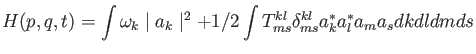
Next, I was asked to derive the four-wave kinetic equation. I derived both the three- and four-wave kinetic equations using Gershgorin’s thesis, and a book by Dr. Victor Lvov named Kolmogorov Spectra of Turbulence as guides. Starting with the three- and four-wave interaction Hamiltonian, I derived the three- and four-wave kinetic equation after much algebraic manipulation. While this process was difficult and I had to rely heavily on the sources that I was given, I was able to complete the derivation, exercising time dependent perturbation theory, basic complex variables, statistics and Dirac delta functions. The Hamiltonian for the four-wave interactions was:

$$H(p,q,t)= \int \omega _k \mid a _k \mid ^2 +1/2 \int T_{ms}^{kl} \delta _{ms}^{kl} a_k^* a_l^* a_m a_s dkdldmds$$ (8)

Lastly, I was required to show the relation between nk and wk. I did this by starting with the Bose-Einstein statistics for an ensemble of indistinguishable bosons. The Bose-Einstein statistics, as I learned from Thermodynamics and Statistical Mechanics class, is the energy distribution on indistinguishable particles in thermal equilibrium. Since this system is in the classical limit, I was able to make the assumption that

$$\hbar < < kT.$$ (9)

Because of this, I was able to prove that

$$nk = (T/wk).$$ (10)

Upon proving this, it became my task to take the system of 128 particles above, and let the system evolve over a long period of time, and check to see if thermal equilibrium was reached. Since (6) was the criterion for thermal equilibrium in the classical regime, it made since that if I plotted

$$log(nk)$$ (11)

versus

$$– log(wk)$$ (12)

I should be able to see and near linear relationship. This is precisely what I did. (See Figure 1).

Figure 1:

One question that was left unresolved was the use of the Bose-Einstein statistics. I was wondering why it was that we didn’t use Maxwell-Boltzmann distribution for the derivation of (5). After all, MB statistics describe the energy distribution of distinguishable particles and is a classical paradigm that both FD and BE statistics go to in the classical limit.

All in all, I had a very rewarding experience this summer studying under Dr. Lvov. Although a lot was demanded out of me, I was able to refine and apply my knowledge of classical mechanics, thermodynamics, and statistics and further develop numerical methods and computing techniques. A research project like this was the perfect opportunity to exercise my knowledge in mathematics and physics beyond the classroom.