Next: Results
Up: Effective Five Wave Hamiltonian
Previous: Introduction
The basic set of equations describing a two-dimensional
potential flow of an ideal incompressible
fluid with a free surface in a gravity field fluid is
the following one:
here  is the shape of a surface,
  is a potential
function of the flow and
is a potential
function of the flow and  - is a gravitational constant.
As was shown by Zakharov in[8],
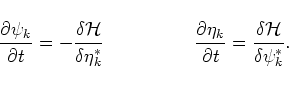
the potential on the surface
- is a gravitational constant.
As was shown by Zakharov in[8],
the potential on the surface
 and are canonically conjugated,
and their Fourier transforms satisfy the equations
and are canonically conjugated,
and their Fourier transforms satisfy the equations
Here
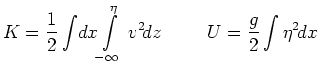
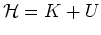 is the total energy of the fluid with the following
kinetic and potential energy terms:
is the total energy of the fluid with the following
kinetic and potential energy terms:
A Hamiltonian can be expanded in an infinite series in powers of
a characteristic wave steepness
 ([,])
by using an iterative procedure. All terms up to the fifth order of this series
contribute to the amplitude of the five-wave interaction.
So the Hamiltonian is expressed in terms of complex wave amplitudes
([,])
by using an iterative procedure. All terms up to the fifth order of this series
contribute to the amplitude of the five-wave interaction.
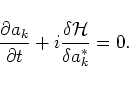
So the Hamiltonian is expressed in terms of complex wave amplitudes  which satisfies the canonical equation of motion:
here
 -is the dispersion law for
the gravity waves.
-is the dispersion law for
the gravity waves.
 can be expanded as follow
 |
|
|
(2.1) |
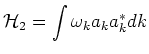
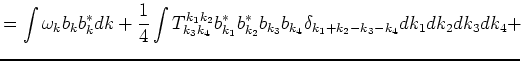
In the normal variable  the second order term in the Hamiltonian
acquires the form:
the second order term in the Hamiltonian
acquires the form:
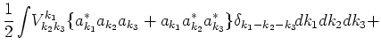
The third order term, which describes
 (first line) and
 processes (second line) is:
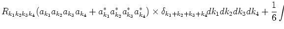
Fourth order term in the Hamiltonian consists of three terms:
describing different types of wave interactions
(first line is
 , second line is
 , last line is
 interactions).
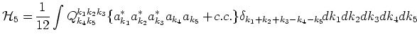
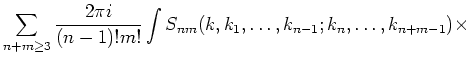
Among the different terms of the fifth order, the only term
corresponding to the process
 is considered:
Here
 are interaction matrix elements of third, fourth and fifth order.
The Hamiltonian
in the normal variables is too complicated to
work with. Our purpose is to simplify the Hamiltonian to the form:
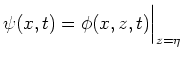
One of the ways to do that is to perform a canonical transformation
[10], [11]
where the  's and
  's are determined
in such a way that the transformation is canonical, and that
the transformed Hamiltonian has the form (2.3).
The transformation (2.4) is canonical up to
the terms of order of
's are determined
in such a way that the transformation is canonical, and that
the transformed Hamiltonian has the form (2.3).
The transformation (2.4) is canonical up to
the terms of order of  .
.
On the resonant manifold
 there are two types of resonances -
trivial and nontrivial. Trivial resonances are
there are two types of resonances -
trivial and nontrivial. Trivial resonances are
 . Nontrivial resonances may be parameterized as
It was shown in [2],[5,6] that on the nontrivial manifold (2.5)
 , i.e. four-wave processes do not produce
``new wave vectors'', and that system is integrable to this degree of accuracy.
This was the main motivation for investigating fifth order interactions.
, i.e. four-wave processes do not produce
``new wave vectors'', and that system is integrable to this degree of accuracy.
This was the main motivation for investigating fifth order interactions.
To find
 one can calculate the terms of the
order of
one can calculate the terms of the
order of  and
and  in the canonical transformation
(2.4). This very cumbersome procedure was fulfilled
by V.Krasitskii[12], but the resulting expressions are so
complicated that they can hardly be used for any practical purpose. Here
the method of Feinman diagrams presented in [13], [1]
is used.
in the canonical transformation
(2.4). This very cumbersome procedure was fulfilled
by V.Krasitskii[12], but the resulting expressions are so
complicated that they can hardly be used for any practical purpose. Here
the method of Feinman diagrams presented in [13], [1]
is used.
First one introduce the so called formal classical scattering matrix which
relates the asymptotic states of the system ``before'' and ``after''
interactions:
By ``for
![$\hat
S[c^{-}_k]$](img48.png) is a nonlinear operator which can be presented
as a series in powers of
is a nonlinear operator which can be presented
as a series in powers of
 .
It has the following form
.
It has the following form
We will treat this series as formal one and will not care about their
convergence [1,14].
The functions
 are the elements of the scattering matrix. They are defined
on the resonant manifolds
are the elements of the scattering matrix. They are defined
on the resonant manifolds
Note, that the value of the matrix element
on the resonant manifold (2.7) is invariant with respect to
the canonical transformation (2.4) and that there is a
simple algorithm for calculation of the matrix elements. The element
is a finite sum of the terms which can be expressed through the
coefficients of the Hamiltonians
 . Each term can be
marked by a certain Feinman diagram taken in a "tree" approximation,
i.e. having no internal loops. To
calculate
one calculates the
first nonzero elements of the scattering matrix
for the Hamiltonian (2.2) and for the Hamiltonian
(2.3). Because these two Hamiltonians are connected by
the canonical transformation (2.4), the results must
coincide.
The first nontrivial element of the scattering matrix in the
one-dimensional case is
. Each term can be
marked by a certain Feinman diagram taken in a "tree" approximation,
i.e. having no internal loops. To
calculate
one calculates the
first nonzero elements of the scattering matrix
for the Hamiltonian (2.2) and for the Hamiltonian
(2.3). Because these two Hamiltonians are connected by
the canonical transformation (2.4), the results must
coincide.
The first nontrivial element of the scattering matrix in the
one-dimensional case is
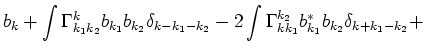
If
 is calculated
in terms of the initial Hamiltonian (2.2)
it consists of 81 terms,
with 60
diagrams combining three third order interactions
(one of such diagrams with
the corresponding expressions is shown below):
is calculated
in terms of the initial Hamiltonian (2.2)
it consists of 81 terms,
with 60
diagrams combining three third order interactions
(one of such diagrams with
the corresponding expressions is shown below):
59#1
and also 20 diagrams combining third-
and fourth order interactions
(one of such diagrams with
the corresponding expressions is shown below):
61#3
and also the fifth order vertex itself.
We use "Mathematica 2.2" for performing the analytical and numerical
calculations of this paper. Initially, the expression for
63#5 occupies 1
Megabyte of computer memory, but we were able to
simplify it to the form presented below. For some of the
orientations, 64#6 is equal to zero. We verify
this fact by
computing
65#7 numerically on 100 random points of the resonant manifold
(3.8) and get zero with accuracy of 66#8.
Next: Results
Up: Effective Five Wave Hamiltonian
Previous: Introduction
Dr Yuri V Lvov
2007-01-17