Boris Gershgorin![]() , Yuri V. Lvov
, Yuri V. Lvov![]() and David Cai
and David Cai![]()
![]() Department of Mathematical Sciences, Rensselaer Polytechnic
Institute, Troy, NY 12180
Department of Mathematical Sciences, Rensselaer Polytechnic
Institute, Troy, NY 12180
The Fermi-Pasta-Ulam (FPU) lattice was introduced in their classical
work [1] to address fundamental issues of statistical physics
such as equipartition of energy, ergodicity. The attempt to resolve
the mystery of the FPU recurrence (the system did not thermalize as
was expected but rather kept returning to the initial
state [1]) has spurred many great mathematical and physical
discoveries, such as the celebrated KAM theorem and soliton
physics [2]. Despite this remarkable progress, there are
still fundamental open questions that are under vigorous
debate [3], such as what is the route to thermalization
and how to fully characterize thermalized ![]() -FPU system.
Furthermore, in the last decade discrete breathers (DB) as spatially
localized, time periodic lattice excitations were
discovered [4]. Arising from energy localization in
nonlinear lattices, they play important roles in many dynamics in
fiber optics, condensed matter physics and molecular
biology [5]. The existence of DBs has been addressed
rigorously [6]. Important conceptual issues
naturally arise, such as what is the role of DBs on the route to
equilibrium [7] and how do they
manifest in thermalization of the FPU system? Resolution of these
issues will certainly provide deep insight into the fundamental
understanding of route to thermalization for general nonlinear
physical systems. Most of the results regarding DBs in
-FPU system.
Furthermore, in the last decade discrete breathers (DB) as spatially
localized, time periodic lattice excitations were
discovered [4]. Arising from energy localization in
nonlinear lattices, they play important roles in many dynamics in
fiber optics, condensed matter physics and molecular
biology [5]. The existence of DBs has been addressed
rigorously [6]. Important conceptual issues
naturally arise, such as what is the role of DBs on the route to
equilibrium [7] and how do they
manifest in thermalization of the FPU system? Resolution of these
issues will certainly provide deep insight into the fundamental
understanding of route to thermalization for general nonlinear
physical systems. Most of the results regarding DBs in ![]() -FPU
chains have so far only addressed their behavior in the transient
state of weakly nonlinear regimes before thermalization
occurs [8,9].
-FPU
chains have so far only addressed their behavior in the transient
state of weakly nonlinear regimes before thermalization
occurs [8,9].
In this Letter, we investigate the FPU dynamics in the strongly
nonlinear limit. We demonstrate that, quite surprisingly, even for
strong nonlinearity, the ![]() -FPU system in thermal equilibrium
behaves like weakly nonlinear waves in properly chosen variables.
Such behavior results from the collective effect of strongly
nonlinear interactions effectively renormalizing linear dispersion
relation. This observation enables us to use a well-developed weak
turbulence (WT) formalism [10] for the description of the
-FPU system in thermal equilibrium
behaves like weakly nonlinear waves in properly chosen variables.
Such behavior results from the collective effect of strongly
nonlinear interactions effectively renormalizing linear dispersion
relation. This observation enables us to use a well-developed weak
turbulence (WT) formalism [10] for the description of the
![]() -FPU chains even in a strongly nonlinear regime. Furthermore,
in addition to the nonlinear waves, we observe the DB excitations in
the thermalized state of
-FPU chains even in a strongly nonlinear regime. Furthermore,
in addition to the nonlinear waves, we observe the DB excitations in
the thermalized state of ![]() -FPU chains. Previously such DBs
were observed only during transient stages towards
thermalization [8]. Here we show via numerical simulation
that DBs actually persist and coexist with renormalized waves
in the thermalized state. Thus, in the thermalized
-FPU chains. Previously such DBs
were observed only during transient stages towards
thermalization [8]. Here we show via numerical simulation
that DBs actually persist and coexist with renormalized waves
in the thermalized state. Thus, in the thermalized ![]() -FPU, there are two
kinds of quasi-particle excitations, one localized in
-FPU, there are two
kinds of quasi-particle excitations, one localized in ![]() -space as
renormalized nonlinear waves/phonons, and the other, localized in
-space as
renormalized nonlinear waves/phonons, and the other, localized in
![]() -space as DBs.
-space as DBs.
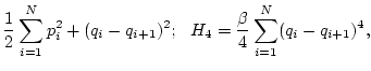
The ![]() -FPU chain is described by the Hamiltonian,
-FPU chain is described by the Hamiltonian,
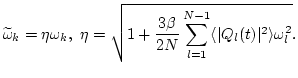
First, for the FPU system in thermal equilibrium [13],
with moderate and strong nonlinearities ![]() and
and ![]() ,
we measured the power spectrum
,
we measured the power spectrum
![]() as a
function of
as a
function of ![]() , where
, where
![]() and
and
![]() denotes the time averaging. Although it was
expected that, for weak
nonlinearity,
denotes the time averaging. Although it was
expected that, for weak
nonlinearity,
![]() , where
, where ![]() is an
effective temperature (Rayleigh-Jeans distribution for
waves [10]), it is surprising to find that the same scaling
holds even for strong nonlinearities as shown in Fig. 1.
To understand why
is an
effective temperature (Rayleigh-Jeans distribution for
waves [10]), it is surprising to find that the same scaling
holds even for strong nonlinearities as shown in Fig. 1.
To understand why
![]() scales as
scales as ![]() even in the strongly
nonlinear limit, we
computed the
even in the strongly
nonlinear limit, we
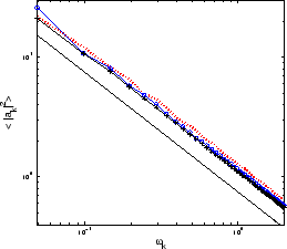
computed the ![]() -
-![]() spectrum of
spectrum of ![]() as shown in
Fig. 2(a). In the weakly nonlinear limit the
spectrum would have resonant peaks along a curve given by the linear
dispersion relation
as shown in
Fig. 2(a). In the weakly nonlinear limit the
spectrum would have resonant peaks along a curve given by the linear
dispersion relation
![]() . We observe that, when the
nonlinearity is no longer small, the
resonances move to higher frequencies, as the dispersion relation is
renormalized by the nonlinear part
. We observe that, when the
nonlinearity is no longer small, the
resonances move to higher frequencies, as the dispersion relation is
renormalized by the nonlinear part ![]() . The renormalized dispersion
relations is
indicated by the sine-like structure of the resonance peaks (the
solid line in Fig. 2(a)). We verified
numerically that the main contribution of the nonlinear potential
energy (
. The renormalized dispersion
relations is
indicated by the sine-like structure of the resonance peaks (the
solid line in Fig. 2(a)). We verified
numerically that the main contribution of the nonlinear potential
energy ( ![]() %) comes from the terms
%) comes from the terms
![]() constrained on
constrained on ![]() . We note that when
. We note that when ![]() and
and ![]() or
or ![]() and
and ![]() , these terms can be combined with the quadratic part of
(2) to effectively renormalize the frequency
, these terms can be combined with the quadratic part of
(2) to effectively renormalize the frequency ![]() .
More specifically, Hamiltonian (2) can be rewritten as
the sum of a new renormalized quadratic part and a remaining
nonlinear part:
.
More specifically, Hamiltonian (2) can be rewritten as
the sum of a new renormalized quadratic part and a remaining
nonlinear part:
![]() where
where
![]() with the renormalized dispersion relation,
with the renormalized dispersion relation,
To further study the renormalization of interactions we measured the
ratio of the quartic to the quadratic parts of the energy
before and after renormalization procedure (i.e.,
![]() vs
vs
![]() ) for different values
of
) for different values
of ![]() with energy fixed (Fig. 2(c)).
This figure also shows that the effective renormalized
linear part becomes more dominant. Therefore even for strongly
nonlinear regimes, with
with energy fixed (Fig. 2(c)).
This figure also shows that the effective renormalized
linear part becomes more dominant. Therefore even for strongly
nonlinear regimes, with ![]() as large as 128, the
renormalized waves (or purely nonlinear phonons) have weakened
interactions. Note that the resonance of
as large as 128, the
renormalized waves (or purely nonlinear phonons) have weakened
interactions. Note that the resonance of ![]() has a finite
width (shown with the dashed lines in Fig. 2(a)
which are the level of
has a finite
width (shown with the dashed lines in Fig. 2(a)
which are the level of
![]() for each
for each
![]() ). We note that for
). We note that for ![]() (the highest mode in the system) the
resonances become the broadest. According to WT [10], the
energy exchange among waves occurs on the resonance manifold given
by
(the highest mode in the system) the
resonances become the broadest. According to WT [10], the
energy exchange among waves occurs on the resonance manifold given
by
![]() and
and
![]() . Although one
can show that there are no exact resonances in
. Although one
can show that there are no exact resonances in ![]() -FPU chains on
the discrete lattice, the nonlinearity induced near resonance interactions (i.e.
-FPU chains on
the discrete lattice, the nonlinearity induced near resonance interactions (i.e.
![]() where
where
![]() is a resonance width) can occur. This allows
us to use the WT theory if the interaction is considered to be weak.
In order to characterize the system as weakly nonlinear waves, the
renormalized waves are described by the new normal variables
is a resonance width) can occur. This allows
us to use the WT theory if the interaction is considered to be weak.
In order to characterize the system as weakly nonlinear waves, the
renormalized waves are described by the new normal variables
![]() The relationship between bare
The relationship between bare ![]() and renormalized
and renormalized
![]() is
is
![]() Under the random phases approximation [14] for
Under the random phases approximation [14] for ![]() we have
we have
![]() Therefore the power spectrum has scaling
Therefore the power spectrum has scaling ![]() for both
for both
![]() and
and
![]() . (Note that
. (Note that
![]() is shown in
Fig. 1).
As a consequence, the effective
temperature,
is shown in
Fig. 1).
As a consequence, the effective
temperature, ![]() , for the renormalized waves, is related
to the bare temperature
, for the renormalized waves, is related
to the bare temperature ![]() by
by
![]() .
.
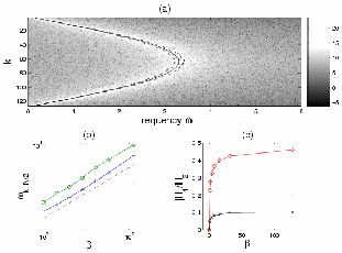
The renormalization picture is further corroborated by the time
evolution of each individual wave
![]() . For the bare
waves
. For the bare
waves ![]() , there are large temporal modulations in both modulus
and phase as a result of strong nonlinear interaction among these
modes on the linear dispersion time scale (as shown in
Fig. 3(a) and (b)). In weakly nonlinear systems, wave
amplitudes and corresponding phases are expected to evolve slowly on
the linear dispersion time scale. For renormalized waves
(Fig. 3(c) and (d))these modes indeed have
characteristics of weakly interacting waves, with a small modulation
in
, there are large temporal modulations in both modulus
and phase as a result of strong nonlinear interaction among these
modes on the linear dispersion time scale (as shown in
Fig. 3(a) and (b)). In weakly nonlinear systems, wave
amplitudes and corresponding phases are expected to evolve slowly on
the linear dispersion time scale. For renormalized waves
(Fig. 3(c) and (d))these modes indeed have
characteristics of weakly interacting waves, with a small modulation
in
![]() and phase.
and phase.
Now we turn to the numerical evidence for the persistence of DBs in
the thermalized ![]() -FPU chain. As observed before [8],
there are DBs present in the transient state. As nonlinearity
increases, the duration of transient becomes shorter. After the
energy redistributes among all the modes to achieve thermal
equilibration, our simulations show that the spatially localized,
high frequency excitations still exist. These DBs can interact with
each other and may be destroyed by collision processes with other
DBs or with the renormalized waves. The spatial structure of these
excitations very much resembles the idealized breather oscillations
in the absence of spatially extended waves: they ``live'' above the
high frequency edge of the dispersion band and their lifetime is
sufficiently long (on the order of 10-100 DB oscillations) to behave
like a quasiparticle. Note that, under certain conditions,
supersonic solitons may arise from the
-FPU chain. As observed before [8],
there are DBs present in the transient state. As nonlinearity
increases, the duration of transient becomes shorter. After the
energy redistributes among all the modes to achieve thermal
equilibration, our simulations show that the spatially localized,
high frequency excitations still exist. These DBs can interact with
each other and may be destroyed by collision processes with other
DBs or with the renormalized waves. The spatial structure of these
excitations very much resembles the idealized breather oscillations
in the absence of spatially extended waves: they ``live'' above the
high frequency edge of the dispersion band and their lifetime is
sufficiently long (on the order of 10-100 DB oscillations) to behave
like a quasiparticle. Note that, under certain conditions,
supersonic solitons may arise from the ![]() -FPU system as another
kind of localized excitations [15,16]. However, they were not
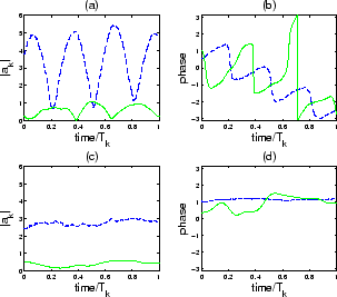
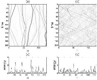
observed in our thermalized system. Fig. 4 is
the energy density plot which shows the time
evolution of energy of each particle for the transient (recording
starting time
-FPU system as another
kind of localized excitations [15,16]. However, they were not
observed in our thermalized system. Fig. 4 is
the energy density plot which shows the time
evolution of energy of each particle for the transient (recording
starting time
![]() ) and thermalized (
) and thermalized (
![]() ) states, respectively. Fig. 4(c) and (d)
display the energy as a function of site at
) states, respectively. Fig. 4(c) and (d)
display the energy as a function of site at ![]() corresponding to
Fig. 4(a) and (b) respectively. In the transient
case (Fig. 4(a)) the spatially localized objects
(dark stripes) that carry sufficiently large amount of energy are
clearly observed. Fig. 4(c) is a snapshot of the
energy density plot (4(a)) at
corresponding to
Fig. 4(a) and (b) respectively. In the transient
case (Fig. 4(a)) the spatially localized objects
(dark stripes) that carry sufficiently large amount of energy are
clearly observed. Fig. 4(c) is a snapshot of the
energy density plot (4(a)) at ![]() . Here the DBs
are seen as localized peaks [8]. After thermalization the
spatial structure looks different (Fig. 4(b)). The
system now consists of the renormalized waves (straight
cross-hatch traces in Fig. 4(b)). On the top of
these waves, the localized structures similar to DBs manifest
themselves as the wavy dark trajectories (in
Fig. 4(b)). Although the snapshot
(Fig. 4(d)) of the energy density plot
(Fig. 4(b)) indicates that in thermal equilibrium
the energy is more evenly distributed among particles, spatially
localized structures are clearly observed.
. Here the DBs
are seen as localized peaks [8]. After thermalization the
spatial structure looks different (Fig. 4(b)). The
system now consists of the renormalized waves (straight
cross-hatch traces in Fig. 4(b)). On the top of
these waves, the localized structures similar to DBs manifest
themselves as the wavy dark trajectories (in
Fig. 4(b)). Although the snapshot
(Fig. 4(d)) of the energy density plot
(Fig. 4(b)) indicates that in thermal equilibrium
the energy is more evenly distributed among particles, spatially
localized structures are clearly observed.
Since there are renormalized waves in the system, which also carry
energy, we need to find a way to distinguish between these waves and
DBs. We use a frequency filter that cuts out the lower side of the
Fourier spectrum and leaves the high frequency part unmodified,
i.e.,
![]() , where
, where ![]() denotes
the real part,
denotes
the real part, ![]() is a time Fourier transform,
is a time Fourier transform, ![]() eliminates all
frequencies below
eliminates all
frequencies below ![]() and
and ![]() is a dynamical variable
that
is being filtered. By applying this filter to the displacement
is a dynamical variable
that
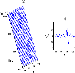
is being filtered. By applying this filter to the displacement ![]() to obtain
to obtain
![]() , we can show the existence of DBs
even for strong nonlinearities, for example,
, we can show the existence of DBs
even for strong nonlinearities, for example, ![]() .
Fig. 5(a) shows a clear
example of a DB excitation reconstructed using the filtered
.
Fig. 5(a) shows a clear
example of a DB excitation reconstructed using the filtered
![]() with
with
![]() . Fig. 5(b) shows
a typical spatial profile of the DB taken from
Fig. 5(a), which strongly resembles the
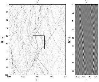
idealized DB [17]. Finally, in Fig. 6, we present the
evidence that there
is a turbulence of DBs, which chaotically ride on renormalized
waves. The corresponding energy density
distribution along with the distribution of filtered displacement in
a zoomed region
. Fig. 5(b) shows
a typical spatial profile of the DB taken from
Fig. 5(a), which strongly resembles the
idealized DB [17]. Finally, in Fig. 6, we present the
evidence that there
is a turbulence of DBs, which chaotically ride on renormalized
waves. The corresponding energy density
distribution along with the distribution of filtered displacement in
a zoomed region ![]() is displayed in Fig. 6(a)
and (b), respectively. After the lower modes from the displacement
is displayed in Fig. 6(a)
and (b), respectively. After the lower modes from the displacement
![]() are filtered, one can clearly observe that the remaining high
frequency oscillations are spatially highly localized, with the same
characteristics as an idealized breather. The detailed time dynamics
of the DB shows the main characteristics of breathers: the
values of
are filtered, one can clearly observe that the remaining high
frequency oscillations are spatially highly localized, with the same
characteristics as an idealized breather. The detailed time dynamics
of the DB shows the main characteristics of breathers: the
values of ![]() change signs periodically (as indicated by the
alternating white and black spots along the trajectory) as the DB
moves in space, with a spatial span of 2 or 3
sites only, as seen in Fig. 6(b).
change signs periodically (as indicated by the
alternating white and black spots along the trajectory) as the DB
moves in space, with a spatial span of 2 or 3
sites only, as seen in Fig. 6(b).
In conclusions, we have presented an interesting
dynamical scenario of the ![]() -FPU chains in thermal equilibrium:
(i) For strong
nonlinearity the linear dispersion relation is effectively
renormalized, which allows one to treat even strongly nonlinear
systems as if
they were weakly nonlinear; (ii) On top of renormalized waves, the strongly nonlinear
system is also characterized by the turbulence of discrete
breathers.
-FPU chains in thermal equilibrium:
(i) For strong
nonlinearity the linear dispersion relation is effectively
renormalized, which allows one to treat even strongly nonlinear
systems as if
they were weakly nonlinear; (ii) On top of renormalized waves, the strongly nonlinear
system is also characterized by the turbulence of discrete
breathers.
Acknowledgments we thank Sergei Nazarenko for discussions.
 |
 |
 |
 |
 |
 |
![$\displaystyle H=\frac{1}{2}\sum_{k=1}^{N-1}\left[\vert P_k\vert^2+\omega_{k}^2\vert Q_k\vert^2\right]+V(Q),$](img16.png)