


Next: Definition of an ideal
Up: Joint statistics of amplitudes
Previous: Introduction
Let us consider a wavefield  in a periodic cube of with
side
in a periodic cube of with
side  and let the Fourier transform of this field be
  where
index
where
index
 marks the mode with wavenumber
 on the grid in the
  -dimensional Fourier space. For
simplicity let us assume that there is a maximum wavenumber
-dimensional Fourier space. For
simplicity let us assume that there is a maximum wavenumber  (fixed e.g. by dissipation) so that no modes with wavenumbers greater
than this maximum value can be excited. In this case, the total
number of modes is
(fixed e.g. by dissipation) so that no modes with wavenumbers greater
than this maximum value can be excited. In this case, the total
number of modes is
 . Correspondingly, index
 will only take values in a finite box,
 which is centred at 0 and all sides of which are equal to
 . To consider homogeneous turbulence, the
large box limit
. To consider homogeneous turbulence, the
large box limit  will have to be taken.
1
will have to be taken.
1
Let us write the complex
 as
as
 where
where  is a real positive
amplitude and
is a real positive
amplitude and  is a phase factor which takes values on
 ,
a unit circle centred at zero in the complex plane. Let us
define the
,
a unit circle centred at zero in the complex plane. Let us
define the  -mode joint PDF
 as the probability for the
wave intensities
as the probability for the
wave intensities  to be in the range
 and for the phase factors to be on the unit-circle
segment between
and for the phase factors to be on the unit-circle
segment between  and
and
 for all
 .
In terms of this PDF, taking the averages
will involve integration over all the real positive
.
In terms of this PDF, taking the averages
will involve integration over all the real positive  's and
along all the complex unit circles of all 's,
's and
along all the complex unit circles of all 's,
 |
|
|
(1) |
where notation  means that
  depends on all
's and all 's in the set
depends on all
's and all 's in the set
 (similarly,
  means
means
 , etc). The full PDF that contains the
complete statistical information about the wavefield
in the infinite
, etc). The full PDF that contains the
complete statistical information about the wavefield
in the infinite  -space can be understood
as a large-box limit
-space can be understood
as a large-box limit
i.e. it is a functional acting on the continuous functions
of the wavenumber,  and
and  .
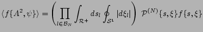
In the the large box
limit there is a path-integral version of (1),
.
In the the large box
limit there is a path-integral version of (1),
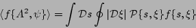 |
(2) |
The full PDF defined above involves all modes (for either
finite or in the limit). By integrating out
all the arguments except for chosen few, one can have
reduced statistical distributions. For example, by
integrating over all the angles and over all but  amplitudes,we have
an ``-mode'' amplitude PDF,
amplitudes,we have
an ``-mode'' amplitude PDF,
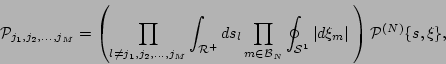 |
(3) |
which depends only on the amplitudes marked by labels
 .
.
Subsections
Next: Definition of an ideal
Up: Joint statistics of amplitudes
Previous: Introduction
Dr Yuri V Lvov
2007-01-17