Phase statistics.

Importantly, RPA formulation involves independent phase factors $\psi = e^\phi$ and not phases $\phi$ themselves. Firstly, the phases would not be convenient because, as we will see later, the mean value of the phases is evolving and one could not say that they are ``distributed uniformly from $-\pi$ to $\pi$''. In fact, we will also see that the mean fluctuation of the phase distribution is also growing and they quickly spread beyond their initial $2 \pi$-wide interval. But perhaps even more important, $\phi$'s build mutual correlations on the nonlinear time whereas $\psi$'s remain independent. This will be shown later in this section, but we would like first to give a simple example illustrating how this property is possible due to the fact that correspondence between $\phi$ and $\psi$ is not a bijection.

Let $N$ be a random integer and let $r_1$ and $r_2$ be two independent (of $N$ and of each other) random numbers with uniform distribution between $-\pi$ and $\pi$. Let

$$\phi_{1,2} = 2 \pi N + r_{1,2}.$$

Then

$$\langle \phi_{1,2}\rangle= 2 \pi \langle N \rangle,$$

and

$$\langle \phi_{1}\phi_{2}\rangle=4\pi^2 \langle N^2 \rangle.$$

Thus,

$$\langle \phi_{1}\phi_{2}\rangle - \langle \phi_{1} \rangle \... ...le = 4 \pi^2 ( \langle N^2 \rangle - \langle N \rangle^2) > 0,$$

which means that variables $\phi_1$ and $\phi_2$ are correlated. On the other hand, if we introduce

$$\psi_{1,2} = e^{i \phi_{1,2}},$$

then

$$\langle \psi_{1,2}\rangle=0,$$

and

$$\langle \psi_{1}\psi_{2}\rangle=0.$$

$$\langle \psi_{1}\psi_{2}\rangle- \langle \psi_{1}\rangle \langle \psi_{2}\rangle =0,$$

which means that variables $\psi_1$ and $\psi_2$ are statistically independent. In this illustrative example it is clear that the difference in statistical properties between $\phi$ and $\psi$ arises from the fact that function $\psi(\phi)$ does not have inverse and, consequently, the information about $N$ contained in $\phi$ is lost in $\psi$.

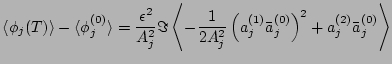
This illustration, although simple, captures the property that actually happens in reality as we will show below. Let us use the following expression for the phase

$$\phi_j = \Im \ln {a_j}.$$

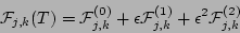
Substituting (8) and Taylor-expanding of logarithm in $\epsilon$ one gets

$$\phi_j = \Im\ln(a_j^{(0)}+{\epsilon}a_j^{(1)}+{\epsilon}^2 a_j^{(2)}) = \phi^{(0)}+{\epsilon}\phi^{(1)}+{\epsilon}^2 \phi^{(2)}$$ (47)

where

$$\phi^{(0)} = \Im\ln a_j^{(0)},$$ (48)

$$\phi^{(1)} = \Im\frac{a_j^{(1)}}{a_j^{(0)}},$$ (49)

$$\phi^{(2)} = \Im\left(-\frac{1}{2}\left(\frac{a_j^{(1)}}{a_j^{(0)}}\right)^2 +\frac{a_j^{(2)}}{a_j^{(0)}}\right).$$ (50)

Now let us perform averaging over the statistics of factors $\psi^{(0)}$. As usual, the surviving terms are those in which all $\psi^{(0)}$'s cancel out due to their pairwise matchings. This is possible only if the number of $\psi^{(0)}$'s is equal to the number of $\bar \psi^{(0)}$'s in the products defining these terms. Easy to see that the ${\epsilon}$ term involves three $\psi^{(0)}$'s and therefore its average is zero. Therefore,

$$\left<\phi_j(T)\right> - \langle\phi^{(0)}_j\rangle = {{\epsilon}... ...\left({a_j^{(1)}}{\bar a_j^{(0)}}\right)^2 + {a_j^{(2)}}{\bar a_j^{(0)}}\right>$$ (51)

Let us consider

$$\left<(a_j^{(1)}\bar a_j^{(0)})^2\right> =\left< \sum_{m,n, \kapp... ...pa a_\kappa \bar a_\nu \bar\Delta_{jn}^m\delta_{j+n}^m\right) \bar a_j^2\right>$$

Here, there are two terms with equal number of $\psi^{(0)}$'s and $\bar \psi^{(0)}$'s but all couplings of index $j$ to any other index give zero because $V=0$ if one of its wavenumbers is zero. Thus, $\left<(a_j^{(1)}\bar a_j^{(0)})^2\right> =0$. The other term, $\left<a_j^{(2)}\bar a_j^{(0)}\right>_\psi$ has already been calculated before when evaluating $J_3$. We have

$$\left<a_j^{(2)}\bar a_j^{(0)}\right>_\psi = 4\sum_{m,n} \left[ - ... ... V_{jn}^m\vert^2 E(0,-\omega_{jn}^m)\delta_{j+n}^m (A_m^2 -A_n^2) \right] A_j^2$$

Let us take limits $N \rightarrow \infty$ and $T \rightarrow \infty$ and replace $\langle \phi(T)\rangle_\psi -\langle \phi(0)\rangle_\psi /T$ by $\dot {\langle \phi \rangle}_\psi$. We get

$$\langle \dot\phi_j \rangle_\psi = \omega_{NL},$$ (52)

where $\omega_{NL}$ is the nonlinear frequency correction given by

$$\omega_{NL} = 4{\epsilon}^2\int \left[\vert V_{mn}^j\vert^2 ... ...} \right) \delta_{j+n}^m(A_m^2-A_n^2)\right]A_j^2 \, dk_m dk_n$$ (53)

Here ${\cal P}(x)$ denotes the principal value of the integral. Averaging over the amplitudes, we have

$$\dot {\langle \phi_j \rangle} = \langle \omega_{NL} \rangle,$$

where $\langle \omega_{NL} \rangle$ is the amplitude-averaged nonlinear frequency correction

$$\langle \omega_{NL} \rangle = 4{\epsilon}^2\int \left[\vert ... ...n}^m} \right) \delta_{j+n}^m(n_m- n_n)\right]n_j \, dk_m dk_n$$ (54)

We can see that the mean value of the phase is steadily changing over the nonlinear time and, therefore, it would be incorrect to assume that the phase ``remains uniformly distributed from $-\pi$ to $\pi$'' even though this could be true for $t=0$. This is one of the reasons why we formulate RPA in terms of $\psi$ and not $\phi$. Indeed, $\psi$ was shown above to stay uniformly distributed on the unit circle over the nonlinear time.

The other reason is that, strictly speaking, $\phi$'s do not stay de-correlated where as $\psi$'s do (as shown before). We already saw in the beginning of this section that this situation is possible due to the fact that the map $\phi \to \psi = e^{i \phi}$ is not a bijection. Let us now study such a buildup in statistical dependence of the phases, let us consider correlator ${\cal F}_{j,k} \equiv \langle(\phi_j-\langle\phi_j\rangle) (\phi_k-\langle\phi_... ...le=\langle\phi_j \phi_{k}\rangle- \langle\phi_j\rangle\langle\ \phi_{k}\rangle.$ At time $T$ we have

$${\cal F}_{j,k}(T)={\cal F}_{j,k}^{(0)}+{\epsilon}{\cal F}_{j,k}^{(1)}+{\epsilon}^2{\cal F}_{j,k}^{(2)}$$ (55)

where

$${\cal F}_{j,k}^{(0)} = \langle\phi_j^{(0)}\phi_k^{(0)}\rangle- \langle\phi_j^{(0)}\rangle\langle\phi_k^{(0)}\rangle,$$

$${\cal F}_{j,k}^{(1)} = \langle\phi_j^{(1)}\phi_k^{(0)}\rangle + \langle\phi_k^{(1)}\phi_j^{(0)}\rangle,$$

$${\cal F}_{j,k}^{(2)} = \langle\phi_j^{(1)}\phi_k^{(1)}\rangle + \langle\phi_j^{(2)}\phi_... ...langle\phi_k^{(0)}\rangle-\langle\phi_k^{(2)}\rangle\langle\phi_j^{(0)}\rangle.$$ (56)

Here, we have taken into account that, as we showed earlier, $\langle\phi_j^{(1)}\rangle =0$. Let us consider the ${\epsilon}$-term ${\cal F}_{j,k}^{(1)}$, e.g.

$$\langle\phi_j^{(1)}\phi_k^{(0)}\rangle = \Im \langle (a_j^{(... ...\bar a_n\bar a_j\phi_k\rangle\bar \Delta_{jn}^m\delta_{j+n}^m$$ (57)

In this expression, we have a factor $\phi_k$ which enters directly and not via the combination $\psi_k = e^{ i \phi_k}$. Potentially, this could greatly complicate the situation because to objects like $\left< \psi_k \phi_k \right>$ knowledge of the statistics of $\psi$ is not sufficient and one needs the full PDF of $\phi_k$. Fortunately, however, this does not cause problems here because, no matter what index is matched to $k$, matching of the two remaining indices results in $V=0$. Therefore, the contribution of the ${\epsilon}$-terms is nill.

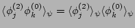
Let us now consider the ${\cal F}_{j,k}^{(2)}$ starting with

$$\langle\phi_j^{(2)}\phi_k^{(0)}\rangle_\psi = \left<\Im\left[-\fr... ...a_j^{(0)})^2 +\frac{1}{A_j^2}a_j^{(2)}\bar a_j^{(0)}\right]\phi_k^{(0)}\right>.$$ (58)

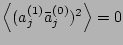
We see that the square bracket on the RHS involves an even number (four or six) of $\psi's$ in each term. Thus, in order for these terms to survive these $\psi's$ must cancel out which is possible when their indices match in a pairwise way. But this means that index $k$ (of $\phi_k$) does not match to any of the indices of $\psi's$ and, therefore, the averaging of $\phi_k$ can be taken separately because it is statistically independent of all other phase factors.⁵Thus, we conclude that $\langle\phi_j^{(2)}\phi_k^{(0)}\rangle_\psi = \langle\phi_j^{(2)}\rangle_\psi \langle \phi_k^{(0)}\rangle_\psi$ and these terms drop out of ${\cal F}_{j,k}^{(2)}$. The remaining term in ${\cal F}_{j,k}^{(2)}$ is

$$\langle\phi_j^{(1)}\phi_k^{(1)}\rangle_\psi = -\frac{1}{4}\left<\left(\frac{a_j^{(1)}}{a_j^{(0)}}-\frac{\bar a_... ...0)}a_k^{(0)}} -\frac{a_j^{(1)}\bar a_k^{(1)}}{a_j^{(0)}a_k^{(0)}} + c.c \right>$$

$$= 2 \vert V_{k(j-k)}^j\vert^2\vert\Delta_{k(j-k)}^j\vert^2 A_{j-k}^... ...{k-j}^2 + {2} \vert V_{jk}^{j+k}\vert^2 \vert\Delta_{jk}^{j+k}\vert^2 A_{j+k}^2$$

$$+ {\delta^j_k \over A_{j}^2} \sum_{l,m} \left[\vert V_{lm}^{j}\vert... ...{jl}^{m}\vert^2 \vert\Delta_{jl}^{m}\vert^2 \delta_{l+j}^{m} \right] A_l^2A_m^2$$ (59)

We can now average over the amplitudes and take limits $N \to \infty$ and ${\epsilon}\to 0$ and write

$$\dot {\cal F}_{j,k} = 4 \pi {\epsilon}^2 \left[ \vert V_{k(j-k)}^j\vert^2 \delta(\omega... ...) n_{k-j} + \vert V_{jk}^{j+k}\vert^2 \delta(\omega_{jk}^{j+k}) n_{j+k} \right]$$

$$+ {2 \pi {\epsilon}^2 \delta^j_k \over n_{j}} \int \left[\vert V_{l... ...}\vert^2 \delta(\omega_{jl}^{m}) \delta_{l+j}^{m} \right] n_l n_m \; dk_l dk_m.$$ (60)

Presence of the 1-st term on the RHS indicates that the phases of the $j$-th and the $k$-th modes get correlated on the nonlinear time. This correlation is week in a sense that ${\cal F}_{j,k}$ has a sharp peak at $j=k$ but the integrated contribution of all $j \ne k$ is of the same order as the value at the contribution of the $j=k$ peak and, therefore, could cause a problem should one tried to build RPA based on the statistics of $\phi$'s rather than $\psi$'s (which remain de-correlated).

Let us consider a special case of (61) for $j=k$ which is interesting because it allows one to calculate the dispersion in phases,

$$\sigma_k = \langle \phi_k^2\rangle - \langle \phi_k\rangle^2$$

We have

$$\dot \sigma_k = \eta_k /n_k,$$ (61)

where $\eta_k$ is defined in (44) and $n_k=\langle \vert a_k\vert^2 \rangle$. One can see that the RHS here is always positive and, therefore, the phase fluctuations experience an unlimited growth. On stationary spectra, this growth is $\sim \sqrt{t}$ which corresponds to $\sigma \sim t$. Recall that the mean value of the phase is also changing in time with the rate $\omega_{NL}$ and on stationary spectra this change is linear in time.