Anomalous probability of large amplitudes in wave turbulence
Physics Letters A,Volume 339, Pages 361-369, 2005

Yeontaek Choi$^*$, Yuri V. Lvov$^\dagger$, Sergey Nazarenko$^*$ and Boris Pokorni$^\dagger$

$^*$ Mathematics Institute, The University of Warwick, Coventry, CV4-7AL, UK
$^\dagger$ Department of Mathematical Sciences, Rensselaer Polytechnic Institute, Troy, NY 12180

Abstract:

Time evolution equation for the Probability Distribution Function (PDF) is derived for system of weakly interacting waves, dominated by the four-wave process. It is shown that a steady state for such system may correspond to strong intermittency.

Introduction -- Wave Turbulence (WT) is a common name for the fields of dispersive waves which are engaged in stochastic weakly nonlinear interactions over a wide range of scales. Numerous examples of WT are found in oceans, atmospheres, plasmas and Bose-Einstein condensates [1,2,3,4,5,6,7,8,9]. For a long time, describing and predicting the energy spectra was the only concern in WT theory. More recently, some attention was given to the study of turbulence intermittency. WT intermittency, or ``burstiness'' of the turbulent signal, was observed experimentally and numerically and was attributed, as in most turbulent systems, to the presence of coherent structures. Examples include collapsing filaments in Bose-Einstein condensates with attractive potentials [9,10], condensate quasi-solitons in systems with repulsive potentials [9,11,12], white caps of sea waves at small scales [13], freak ocean waves at larger scales [14]. Often, such coherent structures are intense but quite sparse so that in most of the space waves remain weakly nonlinear and mostly unaffected by these structures.

Recent analysis of the higher order cumulants [15] showed that WT becomes strongly non-Gaussian at the same length scale where it fails to be weakly nonlinear. In scale invariant systems, the ratio of nonlinear time to the linear wave period grows as a power-law either in to small or toward large wavenumbers. When this growth coincides with the cascade direction then one expects the WT breakdown if the inertial range is large enough. Otherwise intermittency never occurs provided that turbulence is weak at the forcing scale [16]. Further, even if a significant non-Gaussianity occurs, it does not in itself imply intermittency because PDF may remain, in principle, of the same order as Gaussian in all of its parts. This motivates us to study PDFs in WT. Study of PDF in WT context can be traced back to as early as the work of Pierls [17], and, latter, in [18,19], who considered waves in anharmonic crystals, a special case of 3-wave systems. Recently, equations for multimode and one-mode PDF's where derived and analyzed for the general case of 3-wave systems [21,20]. PDF's of the three wave systems were also studied to explain entropy production in three-wave turbulence systems [22]. In the present paper, we will be concerned with the 4-wave case. We are also motivated by a puzzling numerical evidence of a low-wavenumber intermittency in the system of water-surface gravity waves [23] whereas the analysis of [15] predicts intermittency at high wave numbers only. Explaining this fact could shed light on the phenomenon of freak waves [14].

The idea of the present letter is based on the observation that even if the ``hard'' breakdown (as in [15]) does not occur, there will always be a part of the PDF tail for which the amplitudes are too high for WT to work. Such a ``mild'' breakdown will modify the PDF tail in a way that may correspond to intermittency. In fact, this case is easier to study analytically because WT still works for most of the PDF and the wave breaking phenomenon can be modeled simply as a phenomenological cutoff of the PDF tail reflecting the fact that no waves exist above the breaking amplitude. The wave breaking causes ``leakage'' and, therefore, a flux in the amplitude space which is the key phenomenon leading to deviations from the Gaussian equilibrium and intermittency. Note an analogy with the well-known k-space fluxes (cascades) corresponding to Kolmogorov turbulence which is qualitatively different from the thermodynamic equilibrium state. In this paper we will derive an equation for the wave amplitude PDF and we will find its steady state solutions corresponding to the finite flux in the amplitude space. Consequently, we will show that the resulting wave fields are intermittent at each wavenumber with an anomalously large probability of the large-amplitude waves.

Definition of RPA fields -- Previously, the random phase approximation (RPA) has typically assumed that the phases evolve much more rapidly than the amplitudes and, therefore, there exist time intervals where the phases are random but the amplitudes are deterministic [1]. However, numerical simulations indicate that the phase and the amplitude vary at the same time scale [25]. Thus, we need to generalize RPA to the case where both the phases and the amplitudes are random quantities. Such generalization was done in [20,21,24] where 3-wave systems were considered. In the present letter, we will be dealing with 4-wave systems.

Let us consider a wavefield $a({\bf x}, t)$ in a periodic box of volume ${\cal V}$ and let the Fourier transform of this field be $a_k$ where $k \in {\cal Z}^d$ and $d$ is the space dimension. Later we take the large box limit in order to consider homogeneous wave turbulence. Let us write complex $a_k$ as $a_k =A_k \psi_k$ where $A_k \in {\cal R}^+$ is the amplitude and $\psi_k \in {\cal S}^1$ is a phase factor (${\cal S}^1$ being the unit circle in the complex plane). We say the wavefield $a_k$ is of the RPA type if all variables in the set $\{ A_k, \psi_k ; k \in {\cal Z}^d \}$ are statistically independent random variables and $\psi_k$'s are uniformly distributed on ${\cal S}^1$. Defined this way RPA refers not only to the phase but also the amplitude statistics and therefore we suggest a slightly different reading of this acronym: ``Random Phase and Amplitude''.

The above properties are sufficient for our WT analysis and yet such fields may be strongly non-Gaussian. Indeed, RPA allows any shape of the PDF for amplitudes $A_{k}$ and, therefore, it will be a good tool for describing intermittency.

Weakly nonlinear evolution -- Consider a weakly nonlinear wavefield dominated by the 4-wave interactions, e.g. the water-surface gravity waves [1,5,7,13], Langmuir waves in plasmas [1,3] and the waves described by the nonlinear Schroedinger equation [9]. In the finite box, we have the following Hamiltonian equations for the Fourier modes of this field,

$$i \dot b_l = \epsilon \sum_{\alpha\mu\nu} { W^{l\alpha}_{\mu... ...\nu e^{i\omega^{l\alpha}_{\mu\nu}t} \delta^{l\alpha}_{\mu\nu}$$ (1)

where $b_l$ is the wave action variable in the interaction representation, $l \in {\cal Z}^d$, $W^{l \alpha} _{\mu \nu} \sim 1$ is an interaction coefficient, $\omega^{l\alpha}_{\mu\nu} = \omega_l+\omega_{\alpha}-\omega_{\mu}-\omega_{\nu}$, $\omega_l$ is the frequency of mode $l$ and $\epsilon \ll 1$ is a nonlinearity parameter. We are going expand in $\epsilon$ and consider the long-time behavior of a wave field, but in order to make such an analysis consistent we have to renormalize the frequency of () as

$$i \dot a_l = \epsilon \sum_{\alpha\mu\nu} { W^{l\alpha}_{\mu... ...{l\alpha}_{\mu\nu}t} \delta^{l\alpha}_{\mu\nu} - \Omega_l a_l,$$ (2)

where $a_l = b_l e^{i \Omega_l t}$, $\Omega_l = 2 \epsilon \sum_\mu W^{l \mu}_{l \mu} \vert A_\mu(0)\vert^2$ is the nonlinear frequency shift arising from self-interactions and $\tilde \omega^{l\alpha}_{\mu\nu} = \omega^{l\alpha}_{\mu\nu} +\Omega_l+\Omega_\alpha-\Omega_\mu-\Omega_\nu$.

For small nonlinearity, the linear time-scale $2 \pi / \omega$ is a lot less than the nonlinear evolution time which (as will be evident below, see e.g. ()) is $2 \pi \epsilon^2/ \omega$. Thus, to filter out fast oscillations at the wave period, let us seek for the solution at an intermediate time $T$ such that $2 \pi / \omega \ll T \ll 1/(\omega \epsilon^2)$. Now let us use a perturbation expansion in small $\epsilon$, $a_l(T)=a_l^{(0)}+\epsilon a_l^{(1)}+\epsilon^2 a_l^{(2)}.$ Substituting this in () we get in the zeroth order a time independent result, $a_l^{(0)}(T)=a_l(0)$. For simplicity, we will write $a_l(0)= a_l$, understanding that a quantity is taken at $T=0$ if its time argument is not mentioned explicitly. 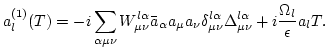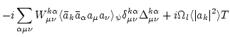The first iteration of () gives

$$a_l^{(1)}(T) = - i \sum_{\alpha\mu\nu} W^{l\alpha}_{\mu\nu} \bar ... ...alpha}_{\mu\nu} \Delta^{l \alpha}_{\mu\nu} + i {\Omega_l \over \epsilon} a_l T.$$ (3)

where

$$\Delta^{l \alpha}_{\mu\nu} \equiv \Delta^{l \alpha}_{\mu\nu}(... ...l\alpha}_{\mu\nu}T}-1})/{i \tilde\omega^{l\alpha}_{\mu\nu}}.$$

Iterating one more time we get

----------------------------------- --

$$a_l^{(2)}(T)=\sum_{\alpha\beta\mu\nu v u}\left( W^{\mu\nu}_{\alph... ...a}, \tilde \omega^{lu}_{v\beta})\right) -\Omega_l^2 a_l \frac{T^2}{2\epsilon^2}$$

$$+ \frac{1}{\epsilon} \sum_{\alpha\mu\nu}\left( \Omega_l W^{l\alph... ...au} d \tau \right) , \hbox{ with } E(x,y)=\int_0^T \Delta(x-y)e^{i y t} d t .$$ (4)

----------------------------------- --

Evolution of statistics -- We will now develop a statistical description via averaging over the initial fields $a_k(0)$ which are taken to be of the RPA type. Of course, to have a non-trivial description valid over the nonlinear evolution time, the fields must remain of the RPA type over the nonlinear time in the leading order in $\epsilon$. The proof of this statement in the 3-wave case was presented in [21,20]. Also [20] contains an announcement of the 4-wave equation for the multi-mode PDF; the details of the relevant analysis will be published separately. Let us introduce a generating function $Z(\lambda ,t)=\langle e^{\lambda \vert a_k(t)\vert^2}\rangle,$ where $\lambda$ is a real parameter. Then PDF of the wave intensities $s= \vert a_k(t)\vert^2$ at each ${\bf k}$ can be written as an inverse Laplace transform, $P(s,t) = \langle \delta (\vert a_k(t)\vert^2 -s) \rangle = {1 \over 2 \pi i} \int_{-i \infty}^{+i \infty} Z(\lambda, t)e^{-s \lambda}d\lambda.$ For the one-point moments we have

$$M_k^{(p)} \equiv \langle \vert a_k\vert^{2p}\rangle =\langle \vert a\vert^{2p}e^{\lambda \vert a\vert^2}\rangle\vert _{\lambda=0}=$$

$$Z_{\lambda \cdots \lambda}\vert _{\lambda=0} = \int_{0}^{\infty} s^p P(s, t) ds,$$ (5)

where $p \in {\cal N}$ and subscript $\lambda$ means differentiation with respect to $\lambda$ $p$ times.

At $t=T$ we have

$$Z(T) = \langle e^{\lambda\vert a_k^{(0)} +\epsilon a_k^{(1)} +\epsilon^2 a_k^{(2)}\vert^2}\rangle = \hspace{1.5cm}$$

$$\langle e^{\lambda \vert a_k^{(0)}\vert^2} \langle 1+\lambda \epsilon (a_k^{(1)} \bar a_k^{(0)}+ {\rm cc})$$

$$\lambda \epsilon^{2}(\vert a_k^{(1)}\vert^{2} + (a_k^{(2)}\bar a_k^{(0)} +{\rm cc}) ) +$$

$${\lambda^2 {\epsilon}^2 \over 2} (a_k^{(1)}\bar a_k^{(0)} +{\rm cc} )^2 \rangle_{\psi} \rangle_{A}$$

$$=Z(0) + {\epsilon}\lambda \langle e^{\lambda \vert a_k^{(0)}\vert^2} \langle a_k^{(1)} \bar a_k^{(0)}+ {\rm cc} \rangle_{\psi} \rangle_{A} +$$

$$\epsilon^{2} \langle \langle (\lambda + \lambda^2 A^2) \vert a_k^{(1)}\vert^{2} + \lambda (a_k^{(2)}\bar a_k^{(0)} +{\rm cc} )$$

$$+ {\lambda^2 \over 2} (a_k^{(1)2} \bar a_k^{(0)2} +{\rm cc}) \rangle_{\psi} \rangle_{A} \hspace{1.5cm}$$ (6)

where ${\rm cc}$ stands for complex conjugate of the previous terms and $\langle\dots\rangle_\psi$ and $\langle\dots\rangle_A$ denote phase and amplitude averaging respectively. Note that in RPA fields the phases and the amplitudes are statistically independent so that these two averaging could be done independently. First let us substitute $a_k^{(1)}$ and $a_k^{(2)}$ from () and () respectively and perform the phase averaging. For the terms proportional to $\epsilon$ we have

$$\langle a_k^{(1)}\bar a_k^{(0)}\rangle_\psi=$$

$$- i \sum_{\alpha\mu\nu} W^{k\alpha}_{\mu\nu} \langle \bar a_k \ba... ...\nu} \Delta^{k \alpha}_{\mu\nu} + i \Omega_l \langle \vert a_k\vert^2 \rangle T$$

$$=- 2 i \sum_{\alpha} W^{k\alpha}_{k\alpha} A_k^2 A_\alpha^2 \cdot T + i \Omega_l A_k^2 T.$$ (7)

where we have used the fact that $\Delta(0)=T$ and we have used the RPA's ``Wick's Theorem''

$$\langle \bar a_k \bar a_\alpha a_\mu a_\nu\rangle_\psi = A_k^... ...delta^k_\mu \delta^\alpha_\nu +\delta^k_\nu\delta^\alpha_\mu).$$

Note that the above expression should also contain the singular cumulant, i.e. term $(A_\alpha^4 - 2A_\alpha^2) \delta^\alpha_\nu \delta^\alpha_\mu \delta^\alpha_k$, see [24]. However we do not write this term here, since its contribution is of the order of $1/N$ smaller because it has one extra delta function.

We see from () that the choice

$$\Omega_k =2 \sum_{\alpha} W^{k\alpha}_{k\alpha} A_\alpha^2$$ (8)

makes the contribution of $\langle a_k^{(1)}\bar a_k^{(0)}\rangle_\psi$ terms to be equal to zero.

We therefore obtain

$$Z(T) -Z(0) = \hspace{2.5cm}$$

$$\lambda \epsilon^{2} \Big\langle \big\langle \lambda \vert a_k^{(... ...+\lambda \vert a_k\vert^2)+ a_k^{(2)}\bar a_k^{(0)} + \bar a_k^{(2)} a_k^{(0)}+$$

$$+\frac{\lambda}{2} ( (\bar a_k^{(0)} a_k^{(1)})^2+{\rm cc}) \big\rangle_{\psi} \Big\rangle_{A}.$$ (9)

where as an intermediate result we have

$$\langle \bar a_k^{(0)} a_k^{(2)}\rangle_\psi=\hspace{2.5cm}$$

$$2\sum\limits_{\alpha \mu\nu} \delta^{k\alpha}_{\mu\nu} \vert W^{k... ... ( A_\mu^2 A_\nu^2 - 2 A_\alpha^2 A_\mu^2) E(0,\tilde\omega^{k\alpha}_{\mu\nu})$$

and

$$\langle \vert\bar a_k^{(1)}\vert^2\rangle_\psi= \sum\limits_{\alp... ...A_\alpha^2 A_\mu^2 A_\nu^2 \vert\Delta(\tilde\omega^{k\alpha}_{\mu\nu})\vert^2.$$

Here terms proportional to $T^2$ drop from $\langle \bar a_k^{(0)} a_k^{(2)}\rangle_\psi$ and $\langle \vert\bar a_k^{(1)}\vert^2\rangle$ because of the choice () of frequency renormalization. Furthermore,

$$\langle (a_k^{(1)}\bar a_k^{(0)})^2 \rangle_\psi=$$

$$-2 W^{k k }_{k k } A_k^6 T^2 \Omega_k -A_k^4 \Omega_k^2 T^2 - 4 \sum_\alpha(W^{k\alpha}_{k\alpha} A_k A_\alpha T )^2$$

To complete the derivation of the equation for the time evolution of the generating function $Z(T)$ we have to take a large box limit, which implies that sums will be replaced with integrals, the Kronecker deltas will be replaced with Dirac's deltas, $\delta^{l \alpha}_{m n}\to\delta^{\alpha l}_{mn}/{\cal V}$, where we introduced short-hand notation, $\delta^{\alpha l}_{mn}=\delta(k_\alpha+k_l-k_m-k_n)$. Then () will still hold, but with

$$\langle \bar a_k^{(0)} a_k^{(2)}\rangle_\psi=\hspace{2.5cm}$$

$$2\int d 123 \delta^{k1}_{23} \vert W^{k1}_{23}\vert^2 A_k^2 ( A_2^2 A_3^2 - 2 A_1^2 A_2^2) E(0,\tilde\omega^{k1}_{23})$$

and

$$\langle \vert\bar a_k^{(1)}\vert^2\rangle_\psi= \int d 123\delta^... ...ert W ^{k1}_{23}\vert^2 A_1 A_2 A_3 \vert\Delta(\tilde\omega^{k1}_{23})\vert^2.$$

We also have

$$\langle (a_k^{(1)}\bar a_k^{(0)})^2 \rangle_\psi = 0,$$ (10)

because this terms will be $1/N$ times smaller than $\langle \vert\bar a_k^{(1)}\vert^2\rangle_\psi$ and $\langle \bar a_k a_k^{(2)}\rangle_\psi$ terms because it has one less summation index. Therefore it vanishes in the $N\to\infty$ limit.

Further we take a large $T$ limit, and take into account that

$$\lim\limits_{T\to\infty}E(0,x)= (\pi \delta(x)+iP(\frac{1}{x})) T,$$

and

$$\lim\limits_{T\to\infty}\vert\Delta(x)\vert^2=2\pi T\delta(x),$$

(see e.g. [2]).

Finally we perform amplitude averaging, noticing that

$$Z(0)=\langle e^{\lambda \vert a_k\vert^2}\rangle_A,$$

and

$$\frac{\partial Z}{\partial \lambda} = \langle \vert a_k\vert^2 e^{\lambda \vert a_k\vert^2} \rangle_A.$$

to obtain

$$Z(T) = Z(0) + \epsilon^2T\cdot( \lambda \eta Z +(\lambda^2 \eta - \lambda \gamma) Z_\lambda).$$ (11)

Approximating $(Z(T)-Z(0))/T$ by $\dot Z$, we have

$$\dot Z = \lambda \eta Z +(\lambda^2 \eta - \lambda n \gamma) Z_\lambda,$$ (12)

where

$$\eta_k = 4 \pi \epsilon^2 \int \vert W^{k1}_{23}\vert^2 \delta^{k1}_{23} \delta(\omega^{k1}_{23}) n_1 n_2 n_3 d123,$$

$$\gamma_k = 8 \pi \epsilon^2 \int \vert W^{k1}_{23}\vert^2 \delta^{k1}_{23} \delta(\omega^{k3}_{12}) \Big[ n_1 (n_2 + n_3) - n_2 n_3\Big] d123,$$

here wavenumbers $k, k_1, k_2, k_3 \in {\cal R}^d$, $\delta$'s now mean Dirac $\delta$-functions, $n_{1,2,3} \equiv n(k_{1,2,3})$ and $d123 = d {\bf k_1} d {\bf k_2} d {\bf k_3}$. Differentiating () with respect to $\lambda$ $p$ times we get the evolution equation for the moments:

$$\dot M^{(p)}_k = -p \gamma_k M^{(p)}_k + p^2 \eta_k M^{(p-1)}_k,$$

which, for $p=1$ gives the standard kinetic equation, $\dot n_k = - \gamma_k n_k + \eta_k .$ First-order PDE () can be easily solved by the method of characteristics. Its steady state solution is

$$Z=(1 -\lambda n_k)^{-1}$$

which corresponds to the Gaussian values of momenta $M^{(p)} = p! n_k^p$. However, these solutions are invalid at small $\lambda$ and high $p$'s because large amplitudes $s=\vert a\vert^2$, for which nonlinearity is not weak, strongly contribute in these cases. Due to the integral nature of definitions of $M^{(p)}$ and $Z$ with respect to the $s=\vert a\vert^2$, the ranges of amplitudes where WT is applicable are mixed with, and contaminated by, the regions where WT fails. Thus, to clearly separate these regions it is better to work with quantities which are local in $s=\vert a\vert^2$, in particular the probability distribution $P(s)$. Taking the inverse Laplace transform of () we have

$$\dot P+\partial_{s}F=0,$$ (13)

where $F=-s(\gamma P+\eta\partial_{s}P)$ is a probability flux in the s-space. Consider the steady state solutions, $\dot P =0$,

$$-s(\gamma P+\eta\partial_{s}P) = F= \hbox{const}.$$ (14)

Note that in the steady state $\gamma /\eta = n_k$ which follows from kinetic equation. The general solution to () is

$$P=P_{hom} + P_{part}$$

where

$$P_{hom} = \hbox{const} \exp{(-s/n)}$$

is the general solution to the homogeneous equation (corresponding to $F=0$) and $P_{part}$ is a particular solution,

$$P_{part} = -({F}/{\eta}) Ei({s}/{n}) \exp{(-s/n)}$$

where $Ei(x)$ is the integral exponential function.

At the tail of the PDF, $s \gg n_k$, the solution can be represented as series in $1/s$, $P_{part} = - F/( s\gamma)-\eta F/(\gamma s)^2+\cdots.$ Thus, the leading order asymptotic of the finite-flux solution is $1/s$ which describes strong intermittency.

Note that if the weakly nonlinearity assumption was valid uniformly to $s=\infty$ then we would have to put $F=0$ to ensure positivity of $P$ and the convergence of its normalization, $\int P ds =1$. In this case $P=P_{hom} = n \exp{(-s/n)}$ which is a pure Rayleigh distribution corresponding to the Gaussian wave field. However, WT approach fails for the amplitudes $s \ge s_{nl}$ for which the nonlinear time is of the same order or less than the linear wave period and, therefore, we can expect a cut-off of $P(s)$ at $s = s_{nl}$. An estimate based on the dynamical equation () gives $s_{nl}= \omega/\epsilon W k^2$. This phenomenological cutoff can be viewed as a wave breaking process which does not allow wave amplitudes to exceed their critical value, $P(s) =0$ for $s > s_{nl}$. Now the normalization condition can be satisfied for the finite-flux solutions. However, having a constant negative flux $F<0$ corresponds to a source at $s = s_{nl}$ which dictates the necessity of a sink for some $s < s_{nl}$ to preserve the normalization of $P(s)$. Note however that the probability sink does not have to correspond to any physical ``removal'' of waves with certain amplitudes. The sink should be present solely because the probability is diluted due to acceptance of new members with $s = s_{nl}$ into the statistical ensemble. In this case, the sink must be proportional to the probability and, taking into account the normalization condition, we can write a modified equation for the PDF in the presence of cutoff,

$$\dot P- \partial_{s} (s\gamma P+s\eta\partial_{s}P)= - F_*,$$ (15)

with $F_* = - P(s_{nl}) \gamma /s_{nl}$. The general solution solution to this equation is $P = [C -{{F_*} } Ei({s}/{n} - \log s)/\eta ] \exp{(-s/n)},$ there constant $C$ is fixed by the normalization condition. This solution is close to the Rayleigh distribution in the PDF core, $s \sim n$, and it has a $1/s$ tail at $n \ll s < s_{nl}$.

Discussion -- We found that the WT intermittency shows as an anomalously high ($\sim 1/s$) probability of the large-amplitude waves whereas at lower amplitudes distribution appears to be close to Rayleigh ($\sim e^{-s/n}$) which corresponds to Gaussian wave fields. We showed that wave breaking is essential for WT intermittency to be present in the system, yet the details of wave breaking are not important. The role of wave breaking is just to ensure that no wave can have amplitude greater than critical value $s_{nl}$. This simple condition leads to huge mathematical consequences as it generates the flux solutions in the amplitude space and therefore creates the $1/s$ intermittency. On the other hand, the amplitude of the $1/s$ tail is not prescribed by WT and will depend on a particular wave breaking mechanisms in a particular system. However, some conclusions about the dependence of the tail amplitude on the physical parameters can be reached using a dimensional arguments.

Consider the classical example of the gravity waves on the surface of deep water. The linear dispersion relation is given by $\omega_k = \sqrt{ g k}$, and the coefficient of nonlinear interaction $W^{k{\bf\alpha}}_{\bf\mu\nu}$ is given in [1]. This system has two power-law steady state solutions. First one is the spectrum corresponding to the direct cascade of energy toward high-wave numbers, $n_k \propto k^{-4}$ [1,4]. Second one is the spectrum corresponding to the inverse cascade of wave action toward the small $k$ values, $n_k\propto k^{-23/6}$. In addition to the gravity constant $g$, the only quantity which determines the state of the system in the direct cascade range is the energy flux ${\cal P}$ whereas in the inverse cascade range - the particle flux $\cal Q$. The PDF tail strength can be characterized by its area which is a dimensionless number and, therefore, has to depend on the relevant dimensionless combinations in the direct and the inverse cascade ranges, ${\cal P}^{2/3} k^{1/3} /g$ and ${\cal Q} k/g$ respectively. Thus, the PDF tail thickness grows with $k$ but its length decreases until it completely disappears at $k \sim k_{nl}$ (equal to $g^3/{\cal P}^2$ and $g/{\cal Q}$ respectively).

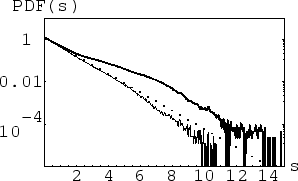
This effect is illustrated in Figure 1 which shows PDF's obtained by numerical simulations of the dynamical equation for surface gravity waves on deep water forced at low $k$'s and dissipated at high $k$'s. Pseudospectral numerical method similar to that of [23],[7] was used on a 256x256 grid. Unlike our study, however, the works in [23],[7] considered unforced turbulence which was freely decaying and unsteady. Note that reaching the long-time steadiness was important for us, in order to accumulate the statistical data necessary for measuring the PDF.

At moderate wavenumber ($k=15 k_{min}$) one can see a PDF tail in the range $4 n_k < s < 10 n_k$ characterized by an order of magnitude enhanced probabilities with respect to the Rayleigh distribution. Unfortunately the range of $s$ where PDF converged to a stable value in this experiment was not large enough to reach $s \gg n$ values and, therefore, for an asymptotic scaling to develop. To increase this range a much longer computing to gain good statistics of very rare events at the PDF tail is necessary, which we can not perform with our resources.

At a higher wavenumber ($k=35 k_{min}$) one can see that the large amplitude waves are less probable than the ones predicted by the Rayleigh distribution. This is because the wave breaking happens now closer to the PDF core causing the PDF cut-off seen at the figure.

In this letter we considered WT which is weak on average so that the wave breaking occurs only in the PDF tail, i.e. $s_{nl} \gg n$. It does not apply to the cases when, at some large $k$, the wave breaking may become so strong that it occurs for most of the waves in the PDF core. These cases where predicted and discussed in [15], but their statistics would be hard to describe analytically because of the strong nonlinearity.

Acknowledgments -- Yeontaek Choi's work is supported by KOSEF M07-2003-000-10003-0. YL is supported by NSF CAREER grant DMS 0134955 and by ONR YIP grant N000140210528

Figure: PDF of $\vert a_k\vert^2$ for $k=15 k_{min}$ (thick curve) and $k=35 k_{min}$ (thin curve) and their comparison with Rayleigh distribution (dotted line). Amplitude s is normalized so that the two curves have the same slope at $s=0$.