Next: Numerical Simulation of Relaxation
Up: Stages of Energy Transfer
Previous: Introduction
Fermi-Pasta-Ulam Model
The Fermi-Pasta-Ulam (FPU) model is a model for a one-dimensional
collection of particles with
massless, weakly anharmonic (nonlinear) springs connecting them to each other.
Letting
 and
and
 denote the
position and momentum coordinates of an
denote the
position and momentum coordinates of an  -particle chain, we can
define the FPU model Hamiltonian:
-particle chain, we can
define the FPU model Hamiltonian:
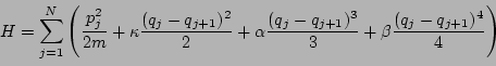 |
(1) |
Here we assumed periodic boundary conditions  and
and
 . Equivalently, the beads are connected in a circular
arrangement. The parameter
. Equivalently, the beads are connected in a circular
arrangement. The parameter  denotes the particle mass, while
  ,
,  , and
, and  are coefficients involving the
spring properties.
are coefficients involving the
spring properties.
The equations of motion are the standard Hamilton's equations:
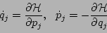 |
(2) |
We will here focus on the -FPU model
for which  and the quartic
term is absent (
and the quartic
term is absent ( ). We nondimensionalize the system
with respect to the spring constant , the mass , and the
energy density
). We nondimensionalize the system
with respect to the spring constant , the mass , and the
energy density  . Retaining
the original symbols for the nondimensionalized variables
. Retaining
the original symbols for the nondimensionalized variables  and
and  ,
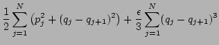
we obtain the nondimensionalized Hamiltonian and equations of motion:
,
we obtain the nondimensionalized Hamiltonian and equations of motion:
Our choice of nondimensionalization implies that
 |
(4) |
for all times.
The fundamental nondimensional parameter measuring the strength of the
nonlinearity is
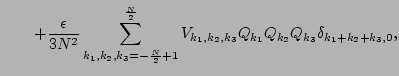
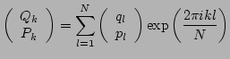
In order to study the transfer of energy among different scales, we
represent the system in terms of Fourier modes:
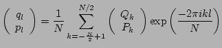 |
|
|
|
 |
|
|
(5) |
The
Hamiltonian in the new variables reads
where the dispersion relation is given by
 |
(7) |
the nonlinear coupling coefficients are
 |
(8) |
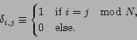
and
is a periodized version of the Kronecker delta function.
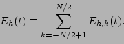
To quantify the amplitude of activity of the FPU chain at different
scales, we define the harmonic energy contribution of each Fourier
mode:
Energy equipartition implies  is independent of
  (and
(and
 ). The total harmonic contribution to the energy is
Next: Numerical Simulation of Relaxation
Up: Stages of Energy Transfer
Previous: Introduction
Dr Yuri V Lvov
2007-01-17
![$\displaystyle \frac{1}{2N}
\sum\limits_{k=-\frac{N}{2}+1}^{\frac{N}{2}}
\left[ \vert P_k\vert^2+\omega_k^2 \vert Q_k\vert^2\right]$](img41.png)